Case study: Application to Austrian COVID-19 survey
We use the methodology developed in Guerrier et al. (2024) to estimate COVID-19 prevalence from a survey conducted in November 2020 by Statistics Austria (2020), and we compare the different estimators to illustrate, in practice, the impact of choosing one method over another.
In November 2020, a survey sample of was collected to test for COVID-19 using PCR tests. Seventy-two participants tested positive; of those, thirty-five () reported having been declared positive by the official procedure during the same month. In November there were declared cases among the approximately Austrian inhabitants over 16 years old, so . The sensitivity () and specificity () are not known with precision, so we present estimates without misclassification error alongside estimates for plausible FP/FN rates consistent with the sensitivities and specificities reported in Kobokovich et al. (2020) and Surkova et al. (2020).
The results presented in Table 2 of Guerrier et al. (2024) can be reproduced as follows:
# Load pempi
library(pempi)

# Austrian data (November 2020)
pi0 = 93914/7166167

# Load data
data("covid19_austria")

# Random sampling
n = nrow(covid19_austria)
R1 = sum(covid19_austria$Y == 1 & covid19_austria$Z == 1)
R2 = sum(covid19_austria$Y == 0 & covid19_austria$Z == 1)
R3 = sum(covid19_austria$Y == 1 & covid19_austria$Z == 0)
R4 = sum(covid19_austria$Y == 0 & covid19_austria$Z == 0)

# Weighted sampling
R1w = sum(covid19_austria$weights[covid19_austria$Y == 1 & covid19_austria$Z == 1])
R2w = sum(covid19_austria$weights[covid19_austria$Y == 0 & covid19_austria$Z == 1])
R3w = sum(covid19_austria$weights[covid19_austria$Y == 1 & covid19_austria$Z == 0])
R4w = sum(covid19_austria$weights[covid19_austria$Y == 0 & covid19_austria$Z == 0])

# Print table
data_mat = matrix(c(R1w, R2w, R3w, R4w, R1, R2, R3, R4), 2, 4, byrow = TRUE)
rownames(data_mat) = c("Weighted sampling", "Unweighted sampling")
colnames(data_mat) = c("R1 (R11)", "R2 (R10)", "R3 (R01)", "R4 (R00)")
knitr::kable(round(data_mat, 4))| R1 (R11) | R2 (R10) | R3 (R01) | R4 (R00) | |
|---|---|---|---|---|
| Weighted sampling | 33.3589 | 0 | 38.2712 | 2218.37 |
| Unweighted sampling | 35.0000 | 0 | 37.0000 | 2218.00 |
The data can be summarized as follows:
- = 2290
- = 1.3105%
-
= 35 (which is denoted as
R1in the package). -
= 33.3589 (which is denoted as
R1orR1win the package). -
= 0 (which is denoted as
R2in the package). -
= 0 (which is denoted as
R2orR2win the package). -
= 37 (which is denoted as
R3in the package). -
= 38.2712 (which is denoted as
R3orR3win the package). -
= 2218 (which is denoted as
R4in the package). -
= 2218.3698 (which is denoted as
R4orR4win the package).
We can check that
R1 + R2 + R3 + R4## [1] 2290and
R1w + R2w + R3w + R4w## [1] 2290For the analysis we consider the possibility of measurement error, in which we use the following values:
# Measurement error
alpha0 = 0
alpha = 1/100
beta = 10/100
Survey MLE
Survey MLE with random sampling
The Survey MLE (with and without measurement error) can be computed as follows and correspond to the numbers reported in Table 3 of Guerrier et al. (2024):
# Survey MLE without measurement error
(smle_no_meas_error_random = survey_mle(R = R1 + R3, n = n))
## Method: Survey MLE
##
## Estimated proportion: 3.1441%
## Standard error : 0.3647%
##
## Confidence intervals at the 95% level:
## Asymptotic Approach: 2.4294% - 3.8588%
## Clopper-Pearson : 2.4680% - 3.9433%
##
## Assumed measurement error: alpha = 0%, beta = 0%
## Sampling: Random
# Survey MLE with measurement error (as defined above)
(smle_with_meas_error_random = survey_mle(R = R1 + R3, n = n,
                              alpha = alpha, beta = beta))
## Method: Survey MLE
##
## Estimated proportion: 2.4091%
## Standard error : 0.4097%
##
## Confidence intervals at the 95% level:
## Asymptotic Approach: 1.6060% - 3.2122%
## Clopper-Pearson : 1.6495% - 3.3070%
##
## Assumed measurement error: alpha = 1%, beta = 10%
## Sampling: RandomSurvey MLE with stratified sampling
In the case of a stratified sampling, the Survey MLE (with and without measurement error) can be computed as follows:
# Survey (weighted) MLE without measurement error
(smle_no_meas_error_strat = survey_mle(R = R1w + R3w, n = n,
                            V = mean(covid19_austria$weights^2)))
## Method: Survey MLE
##
## Estimated proportion: 3.1280%
## Standard error : 0.4471%
##
## Confidence interval at the 95% level:
## Asymptotic Approach: 2.2517% - 4.0042%
##
## Assumed measurement error: alpha = 0%, beta = 0%
## Sampling: Stratified with V = 1.51
# Survey MLE with measurement error (as defined above)
(smle_with_meas_error_strat = survey_mle(R = R1w + R3w, n = n,
                             alpha = alpha, beta = beta,
                             V = mean(covid19_austria$weights^2)))
## Method: Survey MLE
##
## Estimated proportion: 2.3910%
## Standard error : 0.5023%
##
## Confidence interval at the 95% level:
## Asymptotic Approach: 1.4064% - 3.3755%
##
## Assumed measurement error: alpha = 1%, beta = 10%
## Sampling: Stratified with V = 1.51Moment-based estimator
Moment-based estimator with random sampling
In the case of a random sampling, the moment-based estimator or MME (with and without measurement error) can be computed as follows:
# MME without measurement error
(mme_no_meas_error_random = moment_estimator(R3 = R3, n = n,
                            pi0 = pi0))
## Method: Moment Estimator
##
## Estimated proportion: 2.9262%
## Standard error : 0.2635%
##
## Confidence intervals at the 95% level:
## Asymptotic Approach: 2.4099% - 3.4426%
## Clopper-Pearson : 2.4506% - 3.5308%
##
## Assumed measurement error: alpha = 0%, beta = 0%,
## alpha0 = 0%
##
## Estimated false negative rate of the
## official procedure: beta0 = 55.21%
## CI at the 95% level: 47.31% - 63.12%
##
## Estimated ascertainment rate:
## pi0/pi = 44.79%
## CI at the 95% level: 36.88% - 52.69%
##
## Sampling: Random
# MME with measurement error (as defined above)
(mme_with_meas_error_random = moment_estimator(R3 = R3, n = n,
                              pi0 = pi0, alpha = alpha,
                              beta = beta, alpha0 = alpha0))
## Method: Moment Estimator
##
## Estimated proportion: 2.0171%
## Standard error : 0.2960%
##
## Confidence intervals at the 95% level:
## Asymptotic Approach: 1.4369% - 2.5973%
## Clopper-Pearson : 1.4827% - 2.6963%
##
## Assumed measurement error: alpha = 1%, beta = 10%,
## alpha0 = 0%
##
## Estimated false negative rate of the
## official procedure: beta0 = 35.03%
## CI at the 95% level: 16.34% - 53.72%
##
## Estimated ascertainment rate:
## pi0/pi = 64.97%
## CI at the 95% level: 46.28% - 83.66%
##
## Sampling: RandomMoment-based estimator with stratified sampling
In the case of a stratified sampling, the MME (with and without measurement error) can be computed as follows and correspond to the numbers reported in Table 3 of Guerrier et al. (2024):
# MME without measurement error
(mme_no_meas_error_strat = moment_estimator(R3 = R3w, n = n,
                          pi0 = pi0,
                          V = mean(covid19_austria$weights^2)))
## Method: Moment Estimator
##
## Estimated proportion: 2.9818%
## Standard error : 0.3292%
##
## Confidence interval at the 95% level:
## Asymptotic Approach: 2.3365% - 3.6270%
##
## Assumed measurement error: alpha = 0%, beta = 0%,
## alpha0 = 0%
##
## Estimated false negative rate of the
## official procedure: beta0 = 56.05%
## CI at the 95% level: 46.54% - 65.56%
##
## Estimated ascertainment rate:
## pi0/pi = 43.95%
## CI at the 95% level: 34.44% - 53.46%
##
## Sampling: Stratified with V = 1.51
# MME with measurement error (as defined above)
(mme_with_meas_error_strat = moment_estimator(R3 = R3w, n = n,
                             pi0 = pi0, alpha = alpha, beta = beta,
                             alpha0 = alpha0,
                             V = mean(covid19_austria$weights^2)))
## Method: Moment Estimator
##
## Estimated proportion: 2.0794%
## Standard error : 0.3699%
##
## Confidence interval at the 95% level:
## Asymptotic Approach: 1.3544% - 2.8045%
##
## Assumed measurement error: alpha = 1%, beta = 10%,
## alpha0 = 0%
##
## Estimated false negative rate of the
## official procedure: beta0 = 36.98%
## CI at the 95% level: 15.00% - 58.95%
##
## Estimated ascertainment rate:
## pi0/pi = 63.02%
## CI at the 95% level: 41.05% - 85.00%
##
## Sampling: Stratified with V = 1.51Conditional MLE
Conditional MLE with random sampling
In the case of a random sampling, the conditional MLE or CMLE (with and without measurement error) can be computed as follows:
# CMLE without measurement error
(cmle_no_meas_error_random = conditional_mle(R1 = R1, R2 = R2,
                            R3 = R3, R4 = R4, pi0 = pi0))
## Method: Conditional MLE
##
## Estimated proportion: 2.9317%
## Standard error : 0.2639%
##
## Confidence interval at the 95% level:
## Asymptotic Approach: 2.4145% - 3.4489%
##
## Assumed measurement error: alpha = 0%, beta = 0%,
## alpha0 = 0%
##
## Estimated false negative rate of the
## official procedure: beta0 = 55.30%
## CI at the 95% level: 47.41% - 63.18%
##
## Estimated ascertainment rate:
## pi0/pi = 44.70%
## CI at the 95% level: 36.82% - 52.59%
##
## Sampling: Random
# CMLE with measurement error (as defined above)
(cmle_with_meas_error_random = conditional_mle(R1 = R1, R2 = R2,
                              R3 = R3, R4 = R4, pi0 = pi0,
                              alpha = alpha, beta = beta,
                              alpha0 = alpha0))
## Method: Conditional MLE
##
## Estimated proportion: 2.0200%
## Standard error : 0.2962%
##
## Confidence interval at the 95% level:
## Asymptotic Approach: 1.4394% - 2.6006%
##
## Assumed measurement error: alpha = 1%, beta = 10%,
## alpha0 = 0%
##
## Estimated false negative rate of the
## official procedure: beta0 = 35.12%
## CI at the 95% level: 16.48% - 53.77%
##
## Estimated ascertainment rate:
## pi0/pi = 64.88%
## CI at the 95% level: 46.23% - 83.52%
##
## Sampling: RandomConditional MLE with stratified sampling
In the case of a stratified sampling, the CMLE (with and without measurement error) can be computed as follows:
# CMLE without measurement error
(cmle_no_meas_error_strat = conditional_mle(R1 = R1w, R2 = R2w,
                            R3 = R3w, R4 = R4w, pi0 = pi0,
                            V = mean(covid19_austria$weights^2)))
## Method: Conditional MLE
##
## Estimated proportion: 2.9841%
## Standard error : 0.3294%
##
## Confidence interval at the 95% level:
## Asymptotic Approach: 2.3385% - 3.6297%
##
## Assumed measurement error: alpha = 0%, beta = 0%,
## alpha0 = 0%
##
## Estimated false negative rate of the
## official procedure: beta0 = 56.08%
## CI at the 95% level: 46.58% - 65.59%
##
## Estimated ascertainment rate:
## pi0/pi = 43.92%
## CI at the 95% level: 34.41% - 53.42%
##
## Sampling: Stratified with V = 1.51
# CMLE with measurement error (as defined above)
(cmle_with_meas_error_strat = conditional_mle(R1 = R1w, R2 = R2w,
                              R3 = R3w, R4 = R4w, n = n, pi0 = pi0,
                              alpha = alpha, beta = beta,
                              alpha0 = alpha0,
                              V = mean(covid19_austria$weights^2)))
## Method: Conditional MLE
##
## Estimated proportion: 2.0831%
## Standard error : 0.3702%
##
## Confidence interval at the 95% level:
## Asymptotic Approach: 1.3574% - 2.8087%
##
## Assumed measurement error: alpha = 1%, beta = 10%,
## alpha0 = 0%
##
## Estimated false negative rate of the
## official procedure: beta0 = 37.09%
## CI at the 95% level: 15.17% - 59.00%
##
## Estimated ascertainment rate:
## pi0/pi = 62.91%
## CI at the 95% level: 41.00% - 84.83%
##
## Sampling: Stratified with V = 1.51Marginal MLE
Marginal MLE with random sampling
In the case of a random sampling, the marginal MLE or MMLE (with and without measurement error) can be computed as follows:
# MMLE without measurement error
(mmle_no_meas_error_random = marginal_mle(R1 = R1, R3 = R3, n = n, pi0 = pi0))
## Method: Marginal MLE
##
## Estimated proportion: 2.9317%
## Standard error : 0.2639%
##
## Confidence interval at the 95% level:
## Asymptotic Approach: 2.4145% - 3.4489%
##
## Assumed measurement error: alpha = 0%, beta = 0%,
## alpha0 = 0%
##
## Estimated false negative rate of the
## official procedure: beta0 = 55.30%
## CI at the 95% level: 47.41% - 63.18%
##
## Estimated ascertainment rate:
## pi0/pi = 44.70%
## CI at the 95% level: 36.82% - 52.59%
##
## Sampling: Random
# MMLE with measurement error (as defined above)
(mmle_with_meas_error_random  = marginal_mle(R1 = R1, R3 = R3, n = n, pi0 = pi0, alpha = alpha, beta = beta, alpha0 = alpha0))
## Method: Marginal MLE
##
## Estimated proportion: 2.0200%
## Standard error : 0.2962%
##
## Confidence interval at the 95% level:
## Asymptotic Approach: 1.4394% - 2.6006%
##
## Assumed measurement error: alpha = 1%, beta = 10%,
## alpha0 = 0%
##
## Estimated false negative rate of the
## official procedure: beta0 = 35.12%
## CI at the 95% level: 16.48% - 53.77%
##
## Estimated ascertainment rate:
## pi0/pi = 64.88%
## CI at the 95% level: 46.23% - 83.52%
##
## Sampling: RandomReplicating Table 3
Table 3 can be replicated as follows:
table2 = matrix(NA, 6, 6)
rownames(table2) = c("SMLE (stratified)", "MME (stratified)", "Estimated beta0 (stratified)", "SMLE (random)", "MME (random)", "Estimated beta0 (random)")
colnames(table2) = c("Estimates (no meas. err.)", "95% CI (low)", "95% CI (high)", "Estimates (with meas. err.)", "95% CI (low)", "95% CI (high)")

table2[1, ] = 100*c(smle_no_meas_error_strat$estimate,
                smle_no_meas_error_strat$ci_asym,
                smle_with_meas_error_strat$estimate,
                smle_with_meas_error_strat$ci_asym)

table2[2, ] = 100*c(mme_no_meas_error_strat$estimate,
                mme_no_meas_error_strat$ci_asym,
                mme_with_meas_error_strat$estimate,
                mme_with_meas_error_strat$ci_asym)

table2[3, ] = 100*c(mme_no_meas_error_strat$beta0,
                mme_no_meas_error_strat$ci_beta0,
                mme_with_meas_error_strat$beta0,
                mme_with_meas_error_strat$ci_beta0)

table2[4, ] = 100*c(smle_no_meas_error_random$estimate,
                smle_no_meas_error_random$ci_asym,
                smle_with_meas_error_random$estimate,
                smle_with_meas_error_random$ci_asym)

table2[5, ] = 100*c(mme_no_meas_error_random$estimate,
                mme_no_meas_error_random$ci_asym,
                mme_with_meas_error_random$estimate,
                mme_with_meas_error_random$ci_asym)
table2[6, ] = 100*c(mme_no_meas_error_random$beta0,
                mme_no_meas_error_random$ci_beta0,
                mme_with_meas_error_random$beta0,
                mme_with_meas_error_random$ci_beta0)

knitr::kable(round(table2, 3))| Estimates (no meas. err.) | 95% CI (low) | 95% CI (high) | Estimates (with meas. err.) | 95% CI (low) | 95% CI (high) | |
|---|---|---|---|---|---|---|
| SMLE (stratified) | 3.128 | 2.252 | 4.004 | 2.391 | 1.406 | 3.375 |
| MME (stratified) | 2.982 | 2.336 | 3.627 | 2.079 | 1.354 | 2.804 |
| Estimated beta0 (stratified) | 56.049 | 46.537 | 65.560 | 36.977 | 15.003 | 58.951 |
| SMLE (random) | 3.144 | 2.429 | 3.859 | 2.409 | 1.606 | 3.212 |
| MME (random) | 2.926 | 2.410 | 3.443 | 2.017 | 1.437 | 2.597 |
| Estimated beta0 (random) | 55.215 | 47.312 | 63.118 | 35.028 | 16.339 | 53.718 |
Comparing prevalence
This figure can be obtained by running the file
pempi/figures/case_study.Rnw. A similar base R version can
be obtained as follows:
pi0 = 93914/7166167
cols = c("#F8766DFF", "#00BFC4FF")
delta = 0.1
cex_pt = 1.5
lwd_ci = 2
pch_mme = 16
pch_smle = 15

plot(NA, xlim = c(0.75, 4.25), ylim = c(1, 4), axes = FALSE, ann = FALSE)
grid()
box()
col_text = "grey60"
cex_text = 0.85
cex_text2 = 0.65
abline(v = c(1.5, 2.5, 3.5), col = col_text)

axis(2)

mtext("Stratified sampling", side = 3, line = 1.75, cex = cex_text, at = 1, col = col_text)
mtext("no measurement error", side = 3, line = 0.75, cex = cex_text2, at = 1, col = col_text)

mtext("Random sampling", side = 3, line = 1.75, cex = cex_text, at = 2, col = col_text)
mtext("no measurement error", side = 3, line = 0.75, cex = cex_text2, at = 2, col = col_text)

mtext("Stratified sampling", side = 3, line = 1.75, cex = cex_text, at = 3, col = col_text)
mtext("with measurement error", side = 3, line = 0.75, cex = cex_text2, at = 3, col = col_text)

mtext("Random sampling", side = 3, line = 1.75, cex = cex_text, at = 4, col = col_text)
mtext("with measurement error", side = 3, line = 0.75, cex = cex_text2, at = 4, col = col_text)

mtext("Prevalence (%)", side = 2, line = 3, cex = 1.15)
abline(h = 100*pi0, lwd = 2, lty = 2)

text(1, 1.18, expression(pi[0]), cex = 1.15)

legend("topright", c("MME", "95% CI",
                    "Survey MLE", "95% CI"),
       bty = "n", col = c(cols[1], cols[1], cols[2], cols[2]),
       lwd = c(NA, lwd_ci, NA, lwd_ci), pch = c(pch_mme, NA, pch_smle, NA),
       pt.cex = 1.5, cex = 0.7)

# 1) Stratified sampling, without ME
points(1 - delta, 100*mme_no_meas_error_strat$estimate, col = cols[1], pch = pch_mme, cex = cex_pt)
lines(c(1, 1) - delta, 100*mme_no_meas_error_strat$ci_asym, col = cols[1], lwd = lwd_ci)

points(1 + delta, 100*smle_no_meas_error_strat$estimate, col = cols[2], pch = pch_smle, cex = cex_pt)
lines(c(1, 1) + delta, 100*smle_no_meas_error_strat$ci_asym, col = cols[2], lwd = lwd_ci)

# 2) Random sampling, without ME
points(2 - delta, 100*mme_no_meas_error_random$estimate, col = cols[1], pch = pch_mme, cex = cex_pt)
lines(c(2, 2) - delta, 100*mme_no_meas_error_random$ci_asym, col = cols[1], lwd = lwd_ci)

points(2 + delta, 100*smle_no_meas_error_random$estimate, col = cols[2], pch = pch_smle, cex = cex_pt)
lines(c(2, 2) + delta, 100*smle_no_meas_error_random$ci_asym, col = cols[2], lwd = lwd_ci)

# 3) Stratified sampling, with ME
points(3 - delta, 100*mme_with_meas_error_strat$estimate, col = cols[1], pch = pch_mme, cex = cex_pt)
lines(c(3, 3) - delta, 100*mme_with_meas_error_strat$ci_asym, col = cols[1], lwd = lwd_ci)

points(3 + delta, 100*smle_with_meas_error_strat$estimate, col = cols[2], pch = pch_smle, cex = cex_pt)
lines(c(3, 3) + delta, 100*smle_with_meas_error_strat$ci_asym, col = cols[2], lwd = lwd_ci)

# 4) Random sampling, with ME
points(4 - delta, 100*mme_with_meas_error_random$estimate, col = cols[1], pch = pch_mme, cex = cex_pt)
lines(c(4, 4) - delta, 100*mme_with_meas_error_random$ci_asym, col = cols[1], lwd = lwd_ci)

points(4 + delta, 100*smle_with_meas_error_random$estimate, col = cols[2], pch = pch_smle, cex = cex_pt)
lines(c(4, 4) + delta, 100*smle_with_meas_error_random$ci_asym, col = cols[2], lwd = lwd_ci)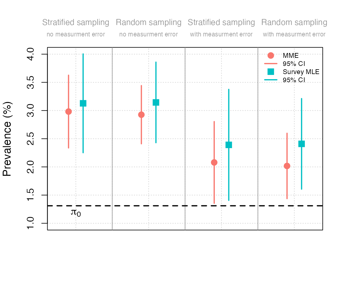
Replicating Figure 1
Figure 1 can be obtained by running the file
pempi/figures/case_study.Rnw. A similar base R version can
be obtained as follows:
# Assumptions
pi0 = 93914/7166167
alpha = 1/100
alpha0 = 0
m = 300
beta = seq(from = 0, to = 30, length.out = m)/100
res_moment = res_smle = matrix(NA, m, 3)
V = mean(covid19_austria$weights^2)

for (i in 1:m){
  # Moment estimator
  inter = moment_estimator(R3 = R3w, n = n, pi0 = pi0,
                           alpha = alpha, alpha0 = alpha0,
                           beta = beta[i], V = V)

  res_moment[i,] = c(inter$estimate, inter$ci_asym)

  # Survey MLE
  inter = survey_mle(R = R1w + R3w, n = n, pi0 = pi0,
                     alpha = alpha, alpha0 = alpha0,
                     beta = beta[i], V = V)

  res_smle[i,] = c(inter$estimate, inter$ci_asym)
}

cols = c("#F8766DFF", "#00BFC4FF")
cols2 = c("#F8766D1F", "#00BFC41F")

plot(NA, xlim = 100*range(beta), ylim = c(1, 4.25), axes = FALSE, ann = FALSE)
grid()
box()
axis(1)
axis(2)
mtext(expression(paste(beta, " (%)")), side = 1, line = 3, cex = 1.15)
mtext("Prevalence (%)", side = 2, line = 3, cex = 1.15)
abline(h = 100*pi0, lwd = 2, lty = 2)
abline(h = 100*pi0, lwd = 2, lty = 2)

text(2.5, 1.18, expression(pi[0]), cex = 1.15)

legend("topleft", c("MME", "95% CI",
                    "Survey MLE", "95% CI"),
       bty = "n", col = c(cols[1], cols2[1],cols[2], cols2[2]),
       lwd = c(3, NA, 3, NA), pch = c(NA, 15, NA, 15),
       pt.cex = 2.5)
lines(100*beta, 100*res_moment[,1], lwd = 3, col = cols[1])
polygon(100*c(beta, rev(beta)),
        100*c(res_moment[,2], rev(res_moment[,3])),
        col = cols2[1], border = NA)

lines(100*beta, 100*res_smle[,1], lwd = 3, col = cols[2])
polygon(100*c(beta, rev(beta)),
        100*c(res_smle[,2], rev(res_smle[,3])),
        col = cols2[2], border = NA)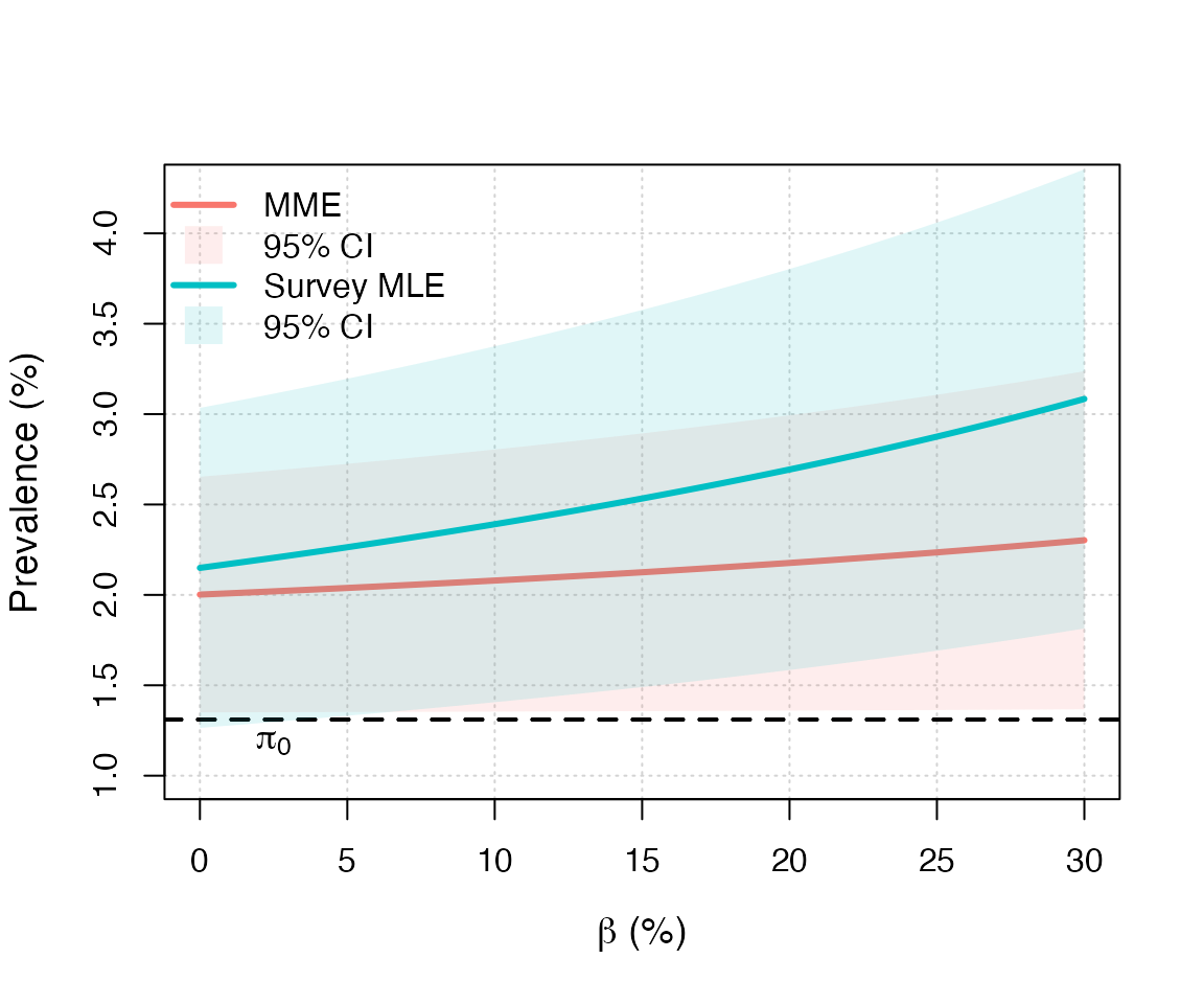
Simulation Study
The results summarized in Section 5 Guerrier et al. (2024) can be replicated as follows:
- Run the file
pempi/simulations/simulation_script.Rwhich should take a couple of hours on a standard laptop (with Monte Carlo replications). This allows to generate the filepempi/simulations/simulations.RData. - Run the file
pempi/simulations/figures.Rnw(which readspempi/simulations/simulations.RData) to generate the figures associated to our simulation study.